

Research Notes: Neural Networks for Baseball
I Have Descended into the Gradients and created SENNA

CAVEAT: I am not an AI expert, nor anything that resembles one. I have zero qualifications to teach you about neural networks. I am NOT confident that all my descriptions are correct, or if what I’ve built is how “real” neural networks are built. In fact, I’m not totally positive that my project even works properly. I’m just a guy who learns through trial and error (one might call my learning process stochastic gradient descent) with the hope, to eventually come out the other side with something useable. Be skeptical of anything you read here and don’t assume I know what I’m talking about. My goal is to inspire you to also dip your toes into this fascinating space.
I suffer greatly from “Not Invented Here Syndrome”. If there’s something that’s been built, that can just be used as is, then it ceases to fascinate me. I always want to push the envelope, break new ground and stretch the art of the possible, all whilst leveraging corporate buzzwords, with a laser focus on baseball, and taking it one neural network at a time.
The majority of baseball models in the public sphere are tree models. Oversimplifying, but they essentially split the data up into buckets, and then decide which bucket your sample fits into. Each of these splits is called a “tree”, with multiple trees combined into an ensemble, weighted and used to make an aggregate prediction. This approach is extremely powerful, and may even outperform a neural network approach.
I began my foray into neural networks by leveraging the fantastic BURN crate. You can dive into it here. For whatever reason (likely user error), I was struggling to get my networks to converge, or make sensible predictions. I spent many (many) fruitless hours tweaking parameters, trying desperately to get something to work. I failed (mostly), but I did not give up, for I have the power of Rust at my disposal. I could just build my own neural network from scratch.
What is a Neural Network?
Neural Networks, for all their complexity, are rather simple structures. Let’s show what a network with precisely 1 “hidden” layer with 2 perceptrons (neurons) looks like. We’ll assume the data set has two inputs, let’s call them Exit Velocity (EV) and Launch Angle (LA), and that we want to predict a continuous result (let’s call it Distance). This is what the network would look like:
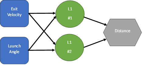
Each of our perceptrons in the green layer connect to our two inputs. The result (Distance) connects to the two green perceptrons.
Each perceptron can be defined by 3 things:
Connections to the previous layer
A bias
An activation function
To caculate L1 #1, we would do the following calculations
EV * Weight 1 + LA * Weight 2
Add a bias
Take the whole number and run it through an activation function
Then the whole idea is to figure out what the correct weights and biases are, as well as figuring out how many perceptrons to have in each layer, as well as how many layers to have.
I could write an entire article on activation functions, but essentially, they add complexity to the network, and ensures your network can’t be collapsed into a single linear function. Traditional networks use a single activation function per layer. The version I built, allows each perceptron to choose its own activation function.
A “hidden” layer (I hate that term) is simply a layer of perceptrons (neurons) that sits between the inputs and the output(s). I dislike the term because it’s not really hidden? My models all output to JSON and you can see all the layers. If I were to name them, I would call them Computation Layers, or Perception Layers.
Stochastic Gradient Descent
Every mathematical function has a derivative. Since the entire network is just a series of mathematical functions, you can calculate the derivative at the end, and then multiply it by the local derivative of every function that it depends on (aka the chain rule). You then move the weights by some multiple of those derivatives (i.e. the “learning rate”. See my caveat at the top!
Vanishing gradients. Certain activation functions or network structures or regularization techniques can cause your gradients to disappear. This is especially true with the ReLU activation function.
Exploding gradients. I think the name speaks for itself.
Learning Rate. The gradient calculated is simply telling you which direction you should adjust the weights. You then need to guess how much to move it. There are a host of research papers on how to do this properly.
Stochastic gradient descent just means that we’re taking a small batch of data to compute the gradients, rather than the entire data set, so the descent is random based on the sample.
When I tried setting up a network using a framework, I would constantly run into issue where the network would just collapse into simply predicting the average result. As I mentioned above, this was likely due to user error.
SENNA
I decided to take the plunge and build a neural network from the ground up. This would allow my to control every aspect of the algorithm, and at the very least deepen my understanding, and in the best case come up with something novel. I have ambititous plans for it - so let’s discuss that first.
Self Evolved Neural Network Architecture
Here’s a rough list of features I plan to build:
Save/Load models to JSON: This is complete. It’s also quite easy to store a history of models, as each model is just a JSON file containing the weights and biases of each perceptron.
Easy data loading from CSV: This was the first thing I completed. Just point at a CSV and tell it which columns you care about.
Regression Models: Create a model that predicts a continous output. The first version of this is complete.
Classification Models: Create a model that classifies inputs into one (or more) possible outputs. I have yet to implement this, but it’s in my pipeline.
Grow/Shrink Layers: This is a tad complicated and my initial attempts at this failed. I want the model to be able to fully evolve itself by shrinking a layer (removing perceptrons), growing layers (adding perceptrons), and theoretically adding and removing entire layers. This solves the problem of having to figure out what the “best” architecture is for a given problem. Ideally, the network should discover this as part of its training.
100% CPU: I don’t know how to leverage a GPU. So I’m calling this a feature, since it allows us to be extremely flexible in how we do things. My workstation has a 3990X 64C/128T CPU, so I really don’t know if this would work for the vast majority of setups.
Flexible Activations: I allow each perceptron to choose its own activation function. This, I think, is a tremendous feature as it allows each layer to have essentially different types of perceptrons, with different methods of firing. I don’t know if that would work well in a GPU-centric architecture, but it’s super easy when you only use CPU.
Deterministic Descent AKA The Optometrist: I remember reading through the BART (Bayesian Additive Regression Trees) research paper(s) and seeing something to the effect of “deterministic error reduction”, where a change is only accepted if it lowers the loss function. This means that after every proposed change, we need check if the network improved. THIS IS VERY COMPUTATIONALLY EXPENSIVE. The reason I call it the Optometrist is it reminds my of what it feels like when the Eye Doc tests your script. "Better or Worse?” they ask, as you shrug and reply “Same”. But each step of the way, the doc is getting closer to your optimal script. Essentially, we tweak weights one by one, allowing the network to gently, slowly, inevitably, find its way. Instead of trying to find a gradient, it just picks a random number and tries to add or subtract it from the weights. This has worked well in a simple data set, but not in a more complex one. I will be experimenting a LOT in this domain. This is essentially a brute force approach.
SENNA Learning


The colour represents the loss function, so you can see how it slowly fits itself to its training data. Here’s the same learning images as a GIF that you absolutely should just watch for hours:
Model Performance
The model maxed out at reducing the loss function to a RMSE of 15.564; if we simply just memoized (fancy word for cached) the distance at each EV and LA, we would get a RMSE of 15.118, so we’re basically only 0.4 feet off the best possible prediction we could hope for. Since we only tweak our network one weight or activation function at a time, we’re at little risk of suddenly over-fitting the data. Here’s how the model views the LA/EV landscape:
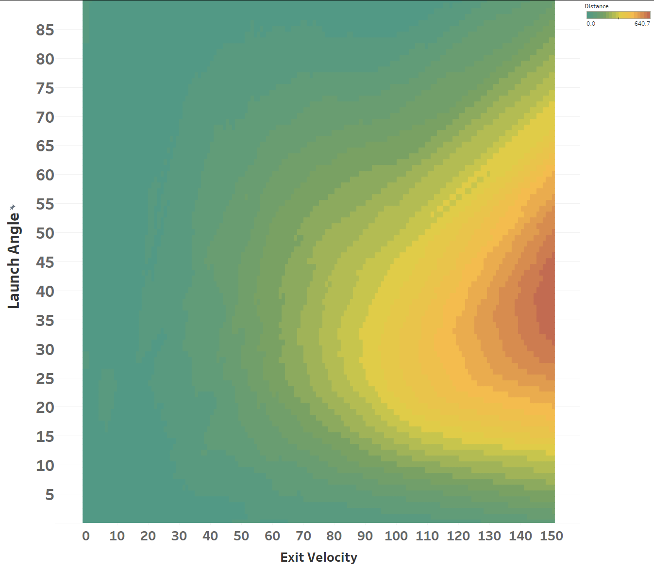
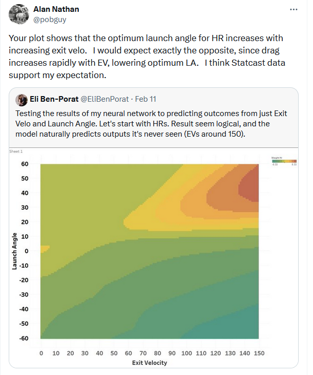
Dr. Nathan (I think) would disagree with the model’s interpretation of the data, as in his view, the optimal launch angle for distance should be lower at higher exit velos. He would probably also caution against using a model to predict things outside of its training data, but I’m mostly presenting this for diagnostic purposes. I’ll post his comments on some of my less-baked work:
I’d take Dr. Nathan’s physics over my neural network, but let’s chart what my model thinks the optimal launch angle is for each Exit Velo. We’ll define optimal as the launch angle which maximizes distance:
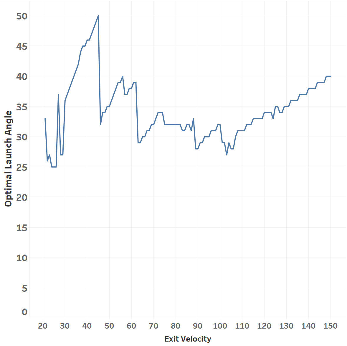
Interestingly, we do see a steady decline in the 50 to 110 range, but a slight uptick in the 110-120 range, which the model then extrapolates out to infinity. This is an important diagnostic as it shows that the model isn’t simply storing results, it’s making actual predictions based on patterns it’s observed in the data. Those observations may be wrong, of course, especially with respect to data it has never seen.
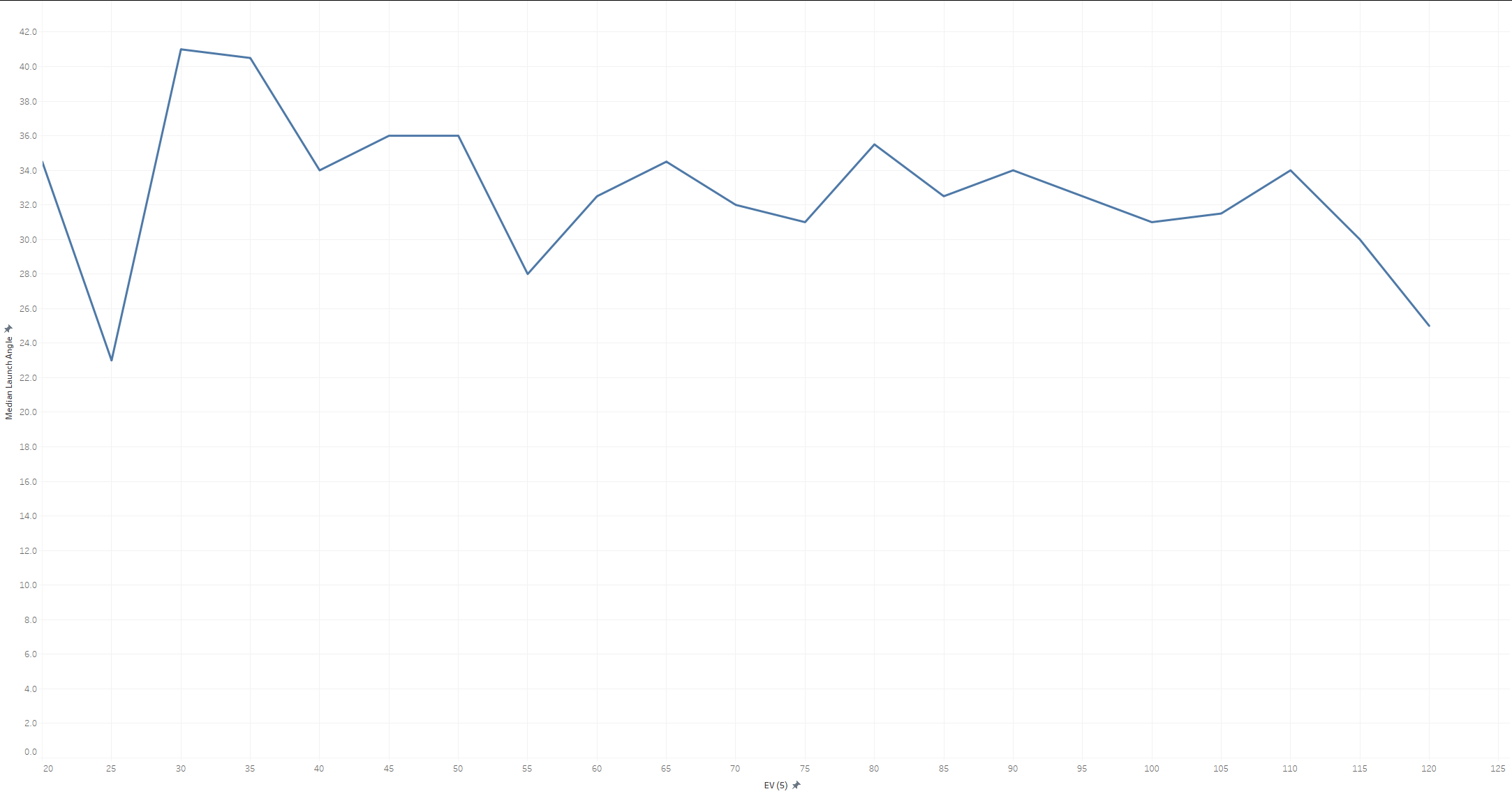
For reference here’s what 2022-2023 look like, which would support Dr. Nathan’s hypothesis:
Concluding Thoughts
My next step is to build a neural network “stuff” model that will absorb a tremendous amount of complexity and attempt to make a bunch of hopefully useful predictions. We’ll see if it bears fruit, but my early results are highly encouraging.